

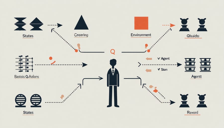
Q-learning stands at the forefront of reinforcement learning, empowering machines to make intelligent decisions through trial and error – much like how humans learn from experience. This powerful algorithm enables AI agents to navigate complex environments, from playing games to controlling robots, without requiring explicit programming for every possible scenario.
At its core, Q-learning builds a decision-making framework by maintaining a table of state-action pairs and their expected rewards. As you build your first AI agent, you’ll discover how it learns to maximize long-term rewards by continuously updating these values based on interactions with its environment.
Unlike traditional programming approaches, Q-learning adapts and improves over time, making it particularly valuable for solving real-world problems where the optimal solution isn’t immediately apparent. Whether you’re a budding AI enthusiast or a seasoned developer, understanding Q-learning opens doors to creating sophisticated AI systems that can learn and evolve autonomously.
This exploration will demystify Q-learning’s fundamental concepts, practical applications, and implementation strategies, equipping you with the knowledge to harness its potential in your own projects.
How Q-Learning Actually Works (Without the Complex Math)
The Reward System Explained
The reward system is the heart of Q-learning, functioning like a sophisticated feedback mechanism that guides the algorithm toward optimal decision-making. Think of it as teaching a pet through treats – good behaviors are rewarded, while unfavorable ones receive no reward or even penalties.
In Q-learning, each action in a given state receives a numerical reward value. These rewards can be positive (encouraging desired behaviors), negative (discouraging unwanted actions), or zero (neutral outcomes). For example, in a maze-solving scenario, reaching the goal might earn a reward of +100, hitting a wall could result in -10, and each regular move might cost -1 to encourage finding the shortest path.
The algorithm uses these rewards alongside a discount factor, which determines how much importance is given to future rewards versus immediate ones. A higher discount factor means the algorithm will prioritize long-term benefits over quick wins, while a lower value focuses on immediate rewards.
What makes this system particularly effective is its ability to learn from both direct and indirect experiences. Even if the immediate reward for an action is small, if it leads to a series of actions with higher cumulative rewards, the algorithm will eventually learn to favor that initial action. This creates a dynamic learning environment where the algorithm continuously updates its understanding of which actions are most valuable in different situations.
Q-Tables: Your AI’s Decision Memory
Think of a Q-table as your AI’s memory book, where it keeps track of what actions worked best in different situations. Just like how you might remember that taking an umbrella when it’s cloudy usually leads to staying dry, a Q-table stores the “quality” or expected reward of taking specific actions in various states.
Imagine you’re teaching a robot to navigate a maze. The Q-table would be organized like a spreadsheet, with each row representing a position in the maze (the state) and each column representing a possible move (the action). At each intersection of state and action, there’s a number – the Q-value – that indicates how good that action is in that situation.
Initially, these Q-values start at zero, like a blank slate. As the AI explores and learns, it updates these values based on the rewards it receives. Higher numbers mean better choices, while lower numbers suggest actions to avoid. For instance, if moving right at a particular junction leads to the exit, that combination of state and action will get a high Q-value.
The beauty of Q-tables lies in their simplicity. They provide a clear, structured way for AI to remember its experiences and make better decisions over time. However, they work best for smaller problems with limited states and actions – when things get more complex, we need more sophisticated approaches.
Setting Up Q-Learning in Collaborative Platforms
Choosing the Right Learning Parameters
Selecting appropriate learning parameters is crucial for successful Q-learning implementation. The two most important parameters are the learning rate (α) and discount factor (γ). Following the right practical implementation steps can help you optimize these values for your specific use case.
The learning rate (α) determines how much new information overrides old information. A value between 0.1 and 0.3 typically works well for most applications. Lower values (closer to 0) make the agent learn slowly but steadily, while higher values (closer to 1) cause rapid learning but may lead to unstable behavior.
The discount factor (γ) balances immediate and future rewards. Values between 0.8 and 0.99 are commonly used. A higher value (closer to 1) makes the agent more forward-thinking, considering future rewards more heavily. Lower values prioritize immediate rewards.
Start with α = 0.1 and γ = 0.9 as baseline values, then adjust based on your agent’s performance. Monitor the learning progress and adjust these parameters if the agent learns too slowly or becomes unstable.
Common Setup Mistakes to Avoid
When implementing Q-learning, several common mistakes can hinder your algorithm’s performance. One frequent error is choosing an inappropriate learning rate. Setting it too high causes unstable learning, while too low makes the learning process unnecessarily slow. Start with a learning rate around 0.1 and adjust based on your specific problem.
Another pitfall is incorrect state representation. Many beginners include unnecessary information in their state space, leading to the curse of dimensionality. Focus on including only relevant features that directly impact the decision-making process.
Poor exploration-exploitation balance is also problematic. Using a static epsilon value throughout training can result in suboptimal policies. Instead, implement an epsilon decay strategy, starting with higher exploration (around 1.0) and gradually decreasing it as the agent learns.
Forgetting to normalize rewards can cause convergence issues. Large reward values can make the Q-values unstable, while tiny values might result in negligible updates. Scale your rewards to a reasonable range, typically between -1 and 1.
Memory management is crucial, especially with large state spaces. Storing every state-action pair in memory isn’t always feasible. Consider using function approximation methods or implementing experience replay with a fixed-size buffer.
Finally, inadequate testing environments can mask problems. Always test your implementation on simple, well-understood problems before tackling complex scenarios. This helps identify and fix issues early in the development process.
Real Projects Using Q-Learning
Game AI Development
Game development provides an excellent playground for implementing Q-learning algorithms, particularly in simple games where the state-action space is manageable. Consider a basic maze game where a character needs to find the shortest path to an exit while avoiding obstacles. In this scenario, Q-learning helps the agent learn optimal movement patterns through trial and error.
One popular example is teaching an AI agent to play Tic-Tac-Toe. The game’s finite state space makes it perfect for Q-learning implementation. The agent learns the value of each possible move by playing thousands of games, gradually building a Q-table that maps game states to optimal actions. Over time, the agent learns to recognize winning strategies and block opponent victories.
Snake is another classic game where Q-learning shines. The agent learns to associate rewards with actions that lead to eating food while avoiding collisions with walls and its own tail. The Q-learning algorithm helps the snake develop increasingly sophisticated strategies, from basic survival to efficient path planning for collecting food.
Grid-world games also demonstrate Q-learning’s effectiveness. In these games, an agent navigates through a grid, collecting rewards while avoiding penalties. The simplicity of the environment makes it easy to visualize how the agent’s decision-making improves as it updates its Q-values based on experiences.
These game implementations serve as stepping stones to understanding more complex applications of Q-learning in advanced game AI and real-world robotics scenarios.

Robotics Training
Q-learning has revolutionized how robots learn and adapt in collaborative environments. Instead of traditional programming where every possible scenario must be explicitly coded, robots using Q-learning can develop their behavior through trial and error, much like humans learn from experience.
In collaborative robot training, Q-learning enables robots to work alongside humans by learning optimal actions for different situations. The robot maintains a Q-table that stores values for various state-action pairs. As it interacts with its environment and human co-workers, it updates these values based on the rewards it receives, gradually improving its decision-making abilities.
For example, in a manufacturing setting, a collaborative robot might learn the best way to hand tools to human workers. Initially, the robot might make mistakes in timing or positioning, but through Q-learning, it discovers which actions lead to successful handovers and which ones cause delays or safety concerns. The robot receives positive rewards for smooth, efficient transfers and negative rewards for actions that interrupt workflow or compromise safety.
Modern robotics platforms often implement Q-learning with safety constraints built into the reward system. This ensures that while the robot is learning autonomously, it maintains strict safety protocols. The learning process typically begins in a simulation environment before moving to real-world applications, allowing the robot to learn from mistakes without risk to human workers or equipment.
This approach has proven particularly effective in flexible manufacturing environments where tasks and conditions frequently change, as the robot can continuously adapt its behavior based on new experiences and feedback.
Optimizing Your Q-Learning Implementation
To get the most out of your Q-learning implementation, several optimization techniques can significantly improve performance and learning efficiency. One key approach is to implement epsilon-greedy exploration with a decay rate. Start with a high epsilon value (around 0.9) and gradually decrease it as the agent learns, allowing for more exploitation of known good actions over time.
Another crucial optimization is proper learning rate adjustment. While a typical starting value is 0.1, you may need to tune this based on your specific problem. A higher learning rate leads to faster learning but might miss optimal solutions, while a lower rate learns more slowly but with greater precision.
Memory management is essential for large state spaces. Consider implementing experience replay, where you store and randomly sample past experiences to train the agent. This helps break action correlations and makes learning more stable. For complex environments, you might want to use prioritized experience replay, giving more weight to important state transitions.
State representation optimization can dramatically impact performance. Rather than using raw state values, normalize your input features to a consistent range (typically 0-1 or -1 to 1). This helps the algorithm converge faster and more reliably.
Don’t forget about reward shaping – the way you structure rewards can significantly affect learning speed. Consider using intermediate rewards to guide the agent toward desired behaviors, rather than only providing rewards at the end of an episode.
Finally, implement proper convergence criteria. Monitor the average reward over time and the Q-value changes. If these metrics stabilize, your agent has likely learned an optimal policy.
Q-learning stands as a powerful foundation for reinforcement learning, offering a practical approach to solving complex decision-making problems. Throughout this exploration, we’ve seen how this algorithm enables agents to learn optimal behaviors through trial and error, without requiring a complete model of their environment.
The key takeaways include understanding the Q-table as a dynamic decision-making tool, the importance of the exploration-exploitation trade-off, and how the learning rate and discount factor influence the algorithm’s performance. We’ve also examined how Q-learning adapts to different scenarios, from simple grid-world problems to sophisticated real-world applications in robotics, game AI, and resource management.
For those looking to implement Q-learning in their projects, start with simple environments to build foundational understanding. Practice implementing the basic algorithm before moving on to more complex variations like Deep Q-learning. Consider joining online communities and participating in reinforcement learning challenges to gain practical experience.
The field of Q-learning continues to evolve, with new developments in areas like multi-agent systems and hybrid approaches combining traditional Q-learning with neural networks. Stay updated with current research and implementations to leverage the full potential of this versatile algorithm.
Remember that mastering Q-learning is an iterative process. Begin with small projects, experiment with different parameters, and gradually tackle more challenging problems as your understanding grows.