
Imagine fine-tuning a piano’s strings – too loose, and the music falls flat; too tight, and the strings might snap. The learning rate in neural networks works similarly, acting as the crucial tuning mechanism that determines how quickly or slowly an AI model adapts to new information. As one of the most critical hyperparameters in modern machine learning techniques, it controls the size of steps a model takes while learning from data.
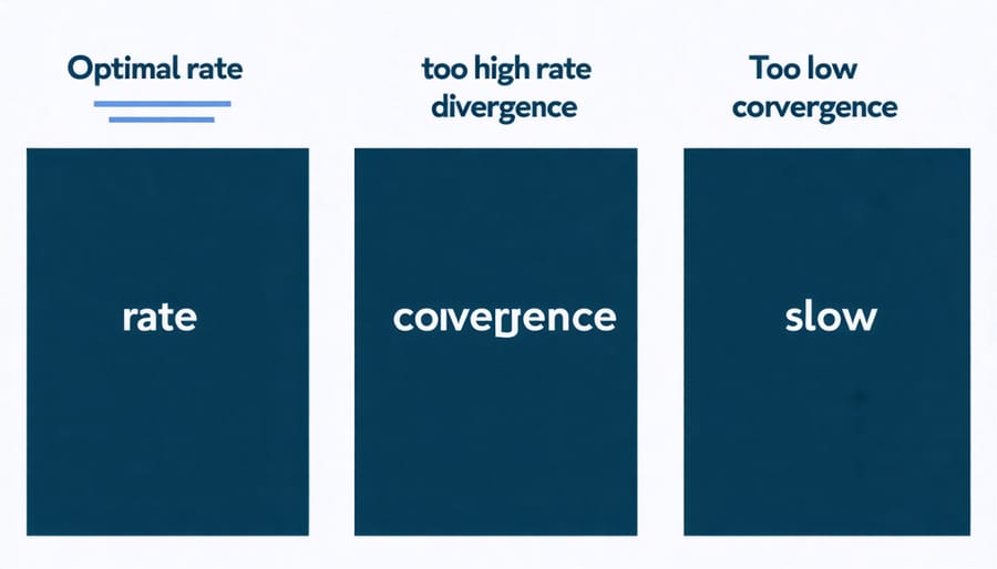
Think of it as the “speed control” for artificial intelligence learning: set it too high, and your model might overshoot optimal solutions, bouncing chaotically between different states; set it too low, and training becomes painfully slow, potentially getting stuck in suboptimal solutions. This delicate balance makes the learning rate a fundamental concept that can mean the difference between a highly accurate model and one that fails to learn effectively.
For data scientists and AI enthusiasts alike, understanding how to tune the learning rate isn’t just about theory – it’s about crafting more efficient, accurate, and reliable neural networks that can tackle real-world problems with precision.
What Makes Learning Rate So Critical?
The Mathematical Magic Behind Learning Rate
Think of learning rate as the size of steps a neural network takes while learning. When updating weights during training, the network uses this formula: New Weight = Old Weight – (Learning Rate × Gradient). The magic lies in how this simple mathematical relationship guides the network toward better performance.
If you’re walking down a hill blindfolded, taking large steps (high learning rate) might get you to the bottom faster, but you risk overshooting or falling. Taking tiny steps (low learning rate) is safer but might make your journey unnecessarily long. Similarly, a learning rate of 0.1 means the network adjusts its weights by 10% of the calculated gradient in each update.
For example, if the gradient suggests a weight should change by 2.0, and your learning rate is 0.01, the actual weight update will be 0.02. This controlled adjustment helps the network find the sweet spot between learning too aggressively and too cautiously, ultimately leading to better model performance.
Remember, while the math might seem complex, the concept is simply about controlling how much your network learns from each training example.

Why Your Model’s Success Depends on the Right Rate
Imagine you’re training a model to recognize cats in photos. With a learning rate that’s too high, your model might repeatedly overshoot the correct answer – like a car with oversensitive steering swerving left and right. Set it too low, and your model crawls toward accuracy at a snail’s pace, potentially taking days instead of hours to train.
Consider a real case from computer vision: when training ResNet models on ImageNet, researchers found that starting with a learning rate of 0.1 and gradually decreasing it led to optimal results. In contrast, using a fixed rate of 0.01 resulted in significantly poorer performance.
Another striking example comes from language processing. GPT models achieve their impressive results partly through careful learning rate scheduling. Starting with a higher rate during initial training helps escape poor local minima, while reducing it later enables fine-tuning of weights for better accuracy.
The key is finding the sweet spot for your specific problem. Modern deep learning frameworks often include tools that can help automatically adjust the learning rate during training, making this process more manageable.
Common Learning Rate Pitfalls (And How to Avoid Them)
Too Fast: The Overshooting Problem
Imagine trying to parallel park a car while pressing the gas pedal too hard – you’ll likely overshoot your target spot. This is exactly what happens when your neural network’s learning rate is too high. Despite modern hardware optimization for neural networks, this remains a common challenge.
When the learning rate is too high, the model takes large steps during training, causing it to jump over the optimal solution. Think of it like playing a game where you’re trying to land on a specific number by rolling dice – but instead of regular dice, you’re forced to use dice with only large numbers. You’ll keep overshooting your target!
This overshooting manifests as unstable training, where the loss function bounces wildly instead of smoothly decreasing. You might notice your model’s performance actually getting worse over time, or the training process failing to converge altogether. Common symptoms include:
– Erratic changes in loss values
– Frequent spikes in error rates
– Model weights becoming extremely large or small
– Training process that never stabilizes
The solution typically involves reducing the learning rate to allow for more precise adjustments. Like carefully easing into that parking spot, smaller steps often lead to better results. Modern practice often includes using adaptive learning rates that automatically adjust based on training progress.
Too Slow: When Your Model Barely Learns
Imagine watching a snail race – that’s what training a neural network with a too-low learning rate feels like. When your learning rate is set too small, your model learns at an agonizingly slow pace, taking far more epochs than necessary to reach its optimal performance.
The telltale signs of a learning rate that’s too low include minimal changes in the loss function across multiple training epochs and accuracy improvements that occur at a glacial pace. For example, if your model’s accuracy only improves by 0.1% after hundreds of iterations, you might be dealing with a learning rate that’s too conservative.
This slow learning isn’t just frustrating – it’s inefficient and potentially problematic. Your model might get stuck in local minima, unable to explore better solutions because it’s taking such tiny steps. Think of it like trying to climb down a valley while only allowing yourself to move an inch at a time – you might never reach the bottom!
Moreover, training with a very low learning rate wastes computational resources and time. In real-world applications, where time and computing power are valuable resources, this can translate into unnecessary costs and delayed project timelines.
To fix this, gradually increase your learning rate while monitoring the training metrics. Look for a sweet spot where learning happens at a reasonable pace without becoming unstable. Remember, the goal is to find a balance between speed and stability.
Choosing the Perfect Learning Rate for Your Network
Start Smart: Initial Learning Rate Selection
Choosing the right initial learning rate is crucial for successful neural network training. Think of it like finding the perfect walking speed – too slow, and you’ll take forever to reach your destination; too fast, and you might trip and fall.
A reliable approach to finding a good initial learning rate is the learning rate range test. Start with a very small learning rate (like 1e-7) and gradually increase it while monitoring the loss. Plot the loss against the learning rate, and you’ll typically see a U-shaped curve. The optimal initial learning rate usually lies at the point where the loss starts decreasing most rapidly.
For most neural networks, these initial learning rates often work well:
– 1e-3 (0.001) for standard neural networks
– 1e-4 (0.0001) for convolutional neural networks
– 3e-4 (0.0003) for transformer models
However, these are just starting points. Consider these factors when selecting your initial rate:
– Dataset size: Larger datasets typically work better with smaller learning rates
– Model architecture: Deep networks usually need smaller rates than shallow ones
– Training objective: Complex tasks might require more conservative rates
A practical tip is to start with 1e-3 and adjust based on training behavior. If the loss is unstable or exploding, decrease the rate by a factor of 10. If learning is too slow, increase it by the same factor.
Remember that modern deep learning frameworks often include automatic learning rate finders, which can save you time in finding the optimal starting point.
Dynamic Learning: Rate Scheduling Techniques
Dynamic learning rate scheduling has become a crucial component in modern neural networks, reflecting the significant evolution of AI systems. Instead of using a fixed learning rate throughout the training process, these techniques automatically adjust the rate based on various factors and training progress.
One popular approach is the step decay schedule, which reduces the learning rate by a fixed percentage after a predetermined number of epochs. For example, you might start with a learning rate of 0.1 and halve it every 30 epochs. This helps the model fine-tune its parameters more precisely as training progresses.
Another effective technique is the exponential decay schedule, where the learning rate decreases continuously according to an exponential function. This creates a smoother transition compared to step decay and can help prevent sudden changes in model behavior.
Adaptive learning rate methods like Adam, RMSprop, and Adagrad take this concept further by adjusting the learning rate individually for each parameter. These algorithms monitor the training progress and automatically modify the learning rate based on the gradient history, making them particularly useful for complex datasets and deep architectures.
Learning rate warmup is another innovative approach where the rate gradually increases from a very small value to the initial learning rate during the first few epochs. This technique helps stabilize training in the crucial early stages when gradients can be particularly volatile.
Cyclical learning rates represent a more recent development, where the learning rate oscillates between a minimum and maximum value. This approach can help the model escape local minima and often leads to better generalization.
Modern Learning Rate Optimization Tools
Popular Learning Rate Optimizers
Modern neural networks benefit from sophisticated learning rate optimizers that automatically adjust the learning rate during training. The most popular among these is Adam (Adaptive Moment Estimation), which combines the benefits of two other optimization techniques: momentum and RMSprop. Adam adapts the learning rate for each parameter individually, making it particularly effective for deep learning tasks.
RMSprop (Root Mean Square Propagation) is another widely-used optimizer that helps prevent the learning rate from becoming too small. It does this by maintaining a moving average of squared gradients, which helps stabilize training and often leads to faster convergence compared to traditional gradient descent.
AdaGrad (Adaptive Gradient Algorithm) adapts the learning rate to each parameter by scaling it inversely with the square root of the sum of all previous squared gradients. This makes it particularly effective for sparse data but can cause the learning rate to become too small over time.
For projects where computational efficiency in AI is crucial, newer optimizers like AdaBelief and Rectified Adam (RAdam) offer improved stability and faster convergence. These optimizers help reduce the need for extensive hyperparameter tuning while maintaining robust training performance.
When choosing an optimizer, consider your specific use case. While Adam is often a safe default choice, some tasks might benefit from the specialized characteristics of other optimizers.
Automated Learning Rate Finding
Finding the perfect learning rate doesn’t have to be a manual process of trial and error. Modern deep learning frameworks offer automated tools that can help identify optimal learning rates efficiently and systematically.
One popular technique is the Learning Rate Finder, introduced by Leslie Smith in the “Cyclical Learning Rates for Training Neural Networks” paper. This method starts with a very small learning rate and gradually increases it while monitoring the model’s loss. The ideal learning rate typically lies just before the point where the loss starts to increase dramatically.
Fast.ai’s implementation of this technique has made it particularly accessible to practitioners. The process involves training the model for a single epoch while exponentially increasing the learning rate. By plotting the loss against the learning rate, you can visually identify the sweet spot where learning is most effective.
Another automated approach is the Learning Rate Range Test, which helps determine both the minimum and maximum learning rates for cyclical learning rate schedules. This test runs your model through a range of learning rates and tracks performance metrics to establish optimal boundaries.
Modern frameworks like TensorFlow and PyTorch also offer built-in learning rate schedulers that can automatically adjust rates during training. These schedulers can implement strategies like step decay, exponential decay, or cosine annealing, taking the guesswork out of learning rate optimization.
These automated tools not only save time but often lead to better results than manual tuning, making them invaluable for both beginners and experienced practitioners.
Understanding the learning rate is crucial for successful neural network training, and we’ve covered its fundamental aspects, from basic concepts to practical implementation strategies. Remember that the learning rate acts as the conductor of your neural network’s learning symphony, determining how quickly and effectively your model adapts to new information.
Key takeaways include the importance of choosing an appropriate initial learning rate, understanding the impact of learning rate on model convergence, and implementing effective learning rate scheduling techniques. We’ve seen how too high or too low learning rates can derail training, making it essential to find that sweet spot for optimal performance.
To continue your journey in mastering neural network training, consider experimenting with different learning rate schedules on various datasets. Start with simple problems and gradually work your way up to more complex scenarios. Tools like TensorBoard can help visualize how learning rate affects your model’s training progress.
Remember that there’s no one-size-fits-all solution when it comes to learning rates. Each project may require different approaches, and the best way to develop intuition is through hands-on practice and experimentation. Stay updated with the latest developments in adaptive learning rate methods, as this field continues to evolve with new research and techniques.
For your next steps, try implementing different learning rate schedulers in your projects and observe their effects on model performance. This practical experience will help solidify your understanding and improve your neural network optimization skills.